This problem is about finding the best path to get from one point (vertices or nodes) to another touring the shortest possible distance, in other words, that the sum of the sections (edges) between two nodes is minimum.
Following there is problem to solve with a python algorithm using an optimization library, therefore you should propose the necessary expressions.
Exercise:
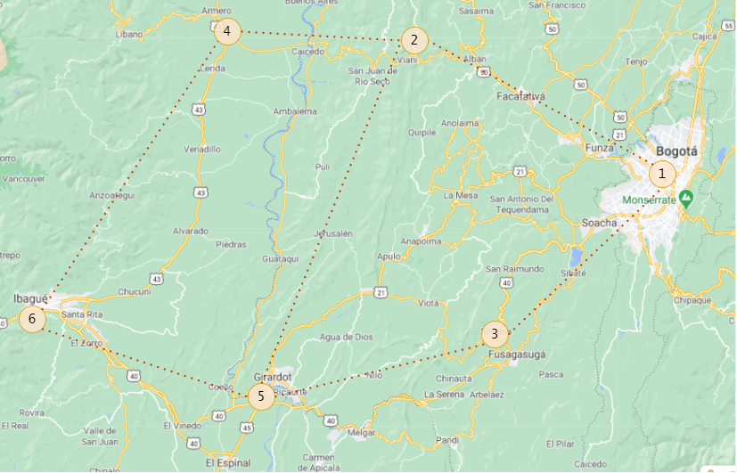
You are in Colombia and want to travel from Bogotá to Ibagué, Tolima for Holy Week. You search the internet for the path you should take and the website shows you in summary a map with 3 possible paths.

- First way: Bogotá-Vianí, Vianí-Armero and Armero-Ibagué
- Second way: Bogotá-Fusagasugá, Fusagasugá-Girardot and Girardot-Ibagué
- Third way: Bogotá-Vianí, Vianí-Girardot and Girardot-Ibagué.
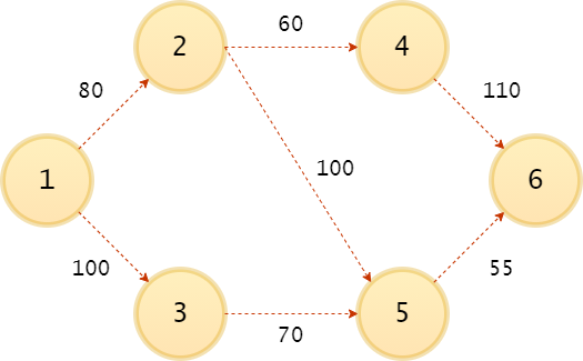
Now observe the graph of the problem, the nodes are the cities or towns, while the sections are the edges with their corresponding value in km.

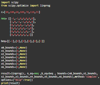
Of the three roads, you must find the shortest to get from Bogotá to Ibagué with the linprog function from the scipy.optimize library and the pseudo-code, however, the required matrices and values must be stated.
import scipy
from scipy.optimize import linprog

#Enter here the variables needed to compile the code

result=linprog(cost list,A_eq=equality constraint matrix,b_eq=equality constraint vector,bounds=(constraint0,constraint1,..,.),method='simplex',options={"disp":True})
#A_eq and b_eq are reserved variables from the library

print(result)
To start all the positions of m columns of the matrices will have the same order for the n rows, that is to say that, if for m = 0 some value of segment X12 (Bogotá-Vianí) is assigned and for m = 1 some value of segment X13 (Bogotá-Fusagasugá) is assigned, so 1 is the reference vertex while 2 and 3 are the node you can arrive at in a single section.
| Pos-m | 0 | 1 | 2 | 3 | 4 | 5 | 6 |
|---|---|---|---|---|---|---|---|
| Segment | X12 | X13 | X24 | X25 | X35 | X46 | X56 |
From this table all variables will be defined: c is a list with the values of each segment between one vertex and the other. In this way, it is added how many meters can be traveled in each of the segments.
| Segment | X12 | X13 | X24 | X25 | X35 | X46 | X56 |
|---|---|---|---|---|---|---|---|
| c | 80 | 100 | 60 | 100 | 70 | 110 | 55 |
Writing the list with Python syntax, c or the cost function will be: $$c=\begin{bmatrix} 80 ,& 100, & 60, & 100, & 70, & 110, & 55 \end{bmatrix} $$
Create a new order to locate the data and write in textarea the c resulting from the change made.
Now the equations of each node with its branches will be raised, taking into account the connections that can be made according to the graph. Through negative or positive binary variables, it is necessary to identify if the point that is taken as a reference reached one of the sections and if they leave with other destinations to new nodes.
Therefore, the row 0 that will store the data of the city or town 1 in the matrix A takes into consideration with whom it shares and with whom it does not, as follows:
| A | B | ||||||||
|---|---|---|---|---|---|---|---|---|---|
| Segment | X12 | X13 | X24 | X25 | X35 | X46 | X56 | SUM | |
| Nod1 | -1 | -1 | 0 | 0 | 0 | 0 | 0 | = | -1 |
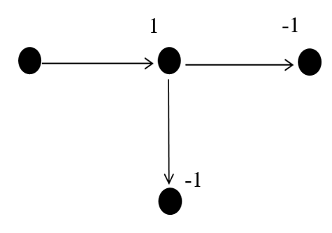
Seeing the city or town as a node in the circuit analysis and the sections as currents, the arrival of a “current” will be represented with a 1, while the exit through the branches with a -1.

However, it does not behave or comply with Kirchhoff's current laws, the input edge is not equal to the sum of the two outputs of the reference node, and according to the problem, one of the options must be chosen to advance, leaving the another at 0, so the result will depend on the sum of the positive or negative binary value of the path that connects to the analyzed node and the path that was chosen to advance to the next city or town. In this way the second row will be:
| A | b | ||||||||
|---|---|---|---|---|---|---|---|---|---|
| Segment | X12 | X13 | X24 | X25 | X35 | X46 | X56 | SUM | |
| Nod1 | -1 | -1 | 0 | 0 | 0 | 0 | 0 | = | -1 |
| Nod2 | 1 | 0 | -1 | -1 | 0 | 0 | 0 | = | 0 |
Complete the expressions for nodes 3, 4, 5, and 6 in the following table and enter the nodes 1 and 2.
Editable NODE Table
From the table the matrix A (7x6) known as the equality restriction matrix and the vector b (6) of equality restrictions will be defined.
According to Python syntax, a 3x3 identity matrix is written as follows:
$$m= \begin{bmatrix}\begin{bmatrix} 1 & 0 & 1 \end{bmatrix},\begin{bmatrix} 0 & 1 & 0 \end{bmatrix},\begin{bmatrix} 0 & 0 & 1 \end{bmatrix}\end{bmatrix} $$
Remember :
$$m=\begin{bmatrix}
1 & 0 & 1\\
0 & 1 & 0\\
0 & 0 & 1
\end{bmatrix}
$$
And a column vector of 3 fields is written as follows: $$v= \begin{bmatrix}\begin{bmatrix} 1 \end{bmatrix},\begin{bmatrix} 1 \end{bmatrix},\begin{bmatrix} 1 \end{bmatrix}\end{bmatrix} $$
Now write matrix A and vector b according to the table you filled out with Python syntax in textarea and use the variable Aeq for the matrix and beq for the vector.
Reviewing the algorithm that is proposed to solve the exercise, the limits or bounds for each node haven’t been defined yet. As the distance traveled from the starting point to the destination proposed in the exercise is positive, a non-negativity restriction must be used, that is, from 0 to infinity.
This is expressed in Python for the starting vertex as:
x0_bounds= (0, None)
Complete the constraints for all vertices.
To obtain the result of the shortest path, you must enter the code shown at the beginning of the exercise in the following console and replace the variables used in this. The result will indicate the total distance of the shortest path, a success message from the compiled code, and the solution path.
Current function value: 225.000000
message: 'Optimization terminated successfully.'
x: array([0., 1., 0., 1., 0., 0., 1.])
.png)