Maximizing or minimizing some function relative to some set, often representing a range of choices available in a certain situation. The function allows comparison of the different choices for determining which might be “best.”
Common applications: Minimal cost, maximal profit, minimal error, optimal design, optimal management, variational principles.
Optimization problems typically have three fundamental elements:
-
The first is a single numerical quantity, or objective function,that is to be maximized or minimizez
-
The second element is a collection of variables, which are quantities whose values can be manipulated in order to optimize the objective
-
The third element of an optimization problem is a set of constraints, which are restrictions on the values that the variables can take
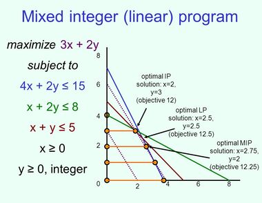
An important class of optimization is known as linear programming. Linear indicates that no variables are raised to higher powers, such as squares. For this class, the problems involve minimizing (or maximizing) a linear objective function whose variables are real numbers that are constrained to satisfy a system of linear equalities and inequalities.

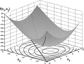
Another important class of optimization is known as nonlinear programming. In nonlinear programming the variables are real numbers, and the objective or some of the constraints are nonlinear functions (possibly involving squares, square roots, trigonometric functions, or products of the variables).

To solve these problems we'll use linprog function from the scipy.optimize library and the pseudo-code, however, the required matrices and values must be stated.

import matplotlib.pyplot as plt
import numpy as np
from scipy.optimize import linprog

c=[]
A_ub=[[],[],[]]
b_ub=[]

#Enter here the variables needed to compile the code

Result=linprog(c,A_ub,b_ub,bounds=(0,None),method='simplex',options={"disp":True})
print(Result)
