Introduction
In this first module, an exercise of nodal analysis of a resistive circuit is presented using Kirchhoff's Law of Currents (KLC). The circuit includes a controlled source in addition to presenting a voltage source between two nodes, defining a supernode between nodes A and B. In this way, this exercise presents such a complete nodal analysis since it integrates the analysis techniques required at this level.
Care must be taken with the directions of the branch currents in the circuit to be able to correctly pose the equations in each of the nodes and finally obtain the correct system of equations.
Once the system of equations is proposed, Python will be used as a tool to facilitate the solution of the system of equations that is expressed in matrix form. Finally, it uses an electronic circuit simulation for contrast system response by measuring variables.
Development
It is proposed for the following circuit, to obtain the values of the current Io and the Vo.
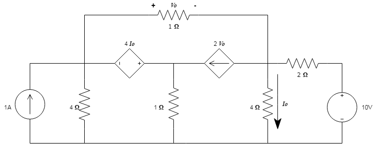
2.1 It is proposed to solve the circuit using the technique of "Nodal analysis." The first thing to do is identify the circuit nodes and proceed to identify them: Va,Vb y Vc.

2.2 Once the nodes have been identified, the control variables are defined based on the node voltages. Obtaining the following equations:
$$Vo=Va-Vc$$ $$Io= \frac {Vc} {4} $$
2.3 Next, the equations of the controlled sources and the equation of the supernode are obtained:
2.3.1 Controlled source equation (4Io)
$$-Va+Vb=4Io$$ $$-Va+Vb=4 \frac {Vc} {4}$$ $$-Va+Vb-Vc=0$$
2.3.2 Supernode equation between *Va* y *Vb*. Kirchhoff's current law is applied in the supernode established between nodes A and B.
$$1 -\frac {Va-Vc}{1}- \frac {Va} {4} -\frac {Vb}{1}+2Vo=0$$ $$1-Va+Vc-\frac {Va}{4}-Vb +2(Va-Vc)=0$$ $$1-Va+Vc-\frac {Va}{4}-Vb +2Va-2Vc=0$$ $$\frac{3}{4} Va-Vb-Vc=-1$$
2.4 Kirchhoff's current law is applied in Vc.
$$ \frac {Va-Vc}{1} -2Vo- \frac {Vc}{4}+\frac{10-Vc}{2}=0$$ $$Va-Vc-2Va+2Vc-\frac {Vc}{4}+5-\frac{ Vc}{2}=0$$ $$-Va+ \frac {Vc}{4}=-5$$
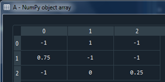
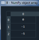
2.5 At this point the system of equations is observed.
$$-Va+Vb-Vc=0$$ $$\frac {3}{4} Va-Vb-Vc=-1$$ $$-Va+\frac{Vc}{4}=-5$$
2.6 To solve this system of equations in Python, the following programming code is implemented.
2.6.1 Python code
2.6.2 To visualize the matrix in Python, assuming that you are working from Spyder, you simply have to "click" on the "play" triangle of the interface, located in the upper part between the middle of the button and the one to execute cell current. After this, the two screens located to the right of the program are observed, the first screen is titled "console" and its function is to display the results of the code: the complex value in rectangular shape and complex value in polar form magnitude and angle in degrees. The second screen has the name "variables explorer" and shows in an organized way in a table, the name of the variables, the type of variable, and the value they have. Furthermore, selecting each of the values obtained shows how data is organized.
2.6 Knowing Va,Vb y Vc, equations are retaken from Io y Vo
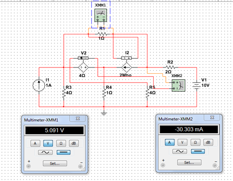
$$Vo=Va-Vc =5.09[v]$$ $$Io=\frac{Vc}{4}=-30.3[mA]$$
2.7 With the help of an electrical circuit simulator, it is verified that the theoretical results coincide with the simulated ones.